import kwant
from matplotlib import pyplot as plt
import tinyarray as ta
import numpy as np
import scipy.sparse.linalg as sla
import scipy


import scipy as scp


from kwant.physics import dispersion
from numpy.linalg import eig
In this notebook we are going to examine some properties of Haldane model of graphen by the use of Kwant package. In the firs step we need to define our system. The crucial idea of defining Haldane model is to introduce complex hopping between next nearest neighbour site. In such a way we make our system gapped in the vicinity od Dirac cones and simultaneously our system stays topologicaly nontrivial.
def make_system_noleads(a=1, t_1=1.0, t_2=1.0, L=10, r=3):
    def circle(pos):
        (x, y) = pos
        rsq = x**2 + y**2
        return rsq < r**2

    R = np.array([[np.sqrt(3) / 2, 1 / 2], [-1 / 2, np.sqrt(3) / 2]])

    v_1 = [3 * a / 2, np.sqrt(3) * a / 2]
    v_2 = [3 * a / 2, -np.sqrt(3) * a / 2]

    r_1 = [0, 0]
    r_2 = [a, 0]

    lat = kwant.lattice.Polyatomic(
        [np.dot(R, v_1), np.dot(R, v_2)], [np.dot(R, r_1), np.dot(R, r_2)], norbs=1
    )

    lat.a, lat.b = lat.sublattices

    syst = kwant.Builder()
    onsite = 0
    # Onsites
    syst[(lat.a(n, m) for n in range(L) for m in range(L))] = onsite
    syst[(lat.b(n, m) for n in range(L) for m in range(L))] = onsite
    # Hopping
    hoppings = (
        ((0, a), lat.a, lat.b),
        ((a, 0), lat.a, lat.b),
        ((-a / 2, -np.sqrt(3) * a / 2), lat.a, lat.b),
        ((-a / 2, np.sqrt(3) * a / 2), lat.a, lat.b),
    )
    syst[[kwant.builder.HoppingKind(*hopping) for hopping in hoppings]] = t_1
    hoppings2_a = (
        ((0, a), lat.a, lat.a),
        ((a, 0), lat.a, lat.a),
        ((a, -a), lat.a, lat.a),
    )

    hoppings2_b = (
        ((0, a), lat.b, lat.b),
        ((a, 0), lat.b, lat.b),
        ((a, -a), lat.b, lat.b),
    )
    syst[[kwant.builder.HoppingKind(*hopping) for hopping in hoppings2_a]] = t_2
    syst[[kwant.builder.HoppingKind(*hopping) for hopping in hoppings2_b]] = t_2

    return syst.finalized()
Topology of the system is strictly related with existance zero mode edge energy states. Using by previously defined system we can picture energy modes in dependently of the parameters values. In the plot below we can observe that for parameters which correspond to the topological phase we have zero energy modes which indeed correspond to edge states.
def SSH_energy(v, w, c):
    syst = make_system_noleads(a=1, t_1=v, t_2=w * np.exp(1j * c), L=5, r=3)
    hamiltonian = syst.hamiltonian_submatrix(sparse=False)
    w1, v1 = eig(hamiltonian)
    plt.plot(np.arange(0, 50, 1), sorted(np.real(w1)), ".")
    plt.axhline(y=0, color="r", linestyle="-")
    plt.show()


SSH_energy(2.5, 2.5, 0)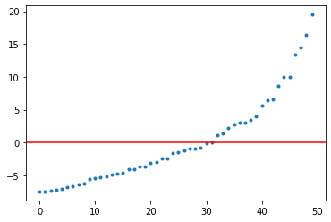
We can go one better and try to plot density of states (DOS). One can observe that indeed fot topological phase ther is clear pics in the vicinity of zero modes.
from mpl_toolkits.axes_grid1.inset_locator import zoomed_inset_axes
from mpl_toolkits.axes_grid1.inset_locator import mark_inset


def x(v, w, c):
    fig, ax = plt.subplots(figsize=[5, 4])
    syst = make_system_noleads(a=1, t_1=v, t_2=w * np.exp(1j * c), L=5, r=3)
    hamiltonian = syst.hamiltonian_submatrix(sparse=False)

    w1, v1 = eig(hamiltonian)
    rho = kwant.kpm.SpectralDensity(hamiltonian, rng=0)
    w1, densities = rho()
    density_subset = np.real(rho(w1))
    ax.plot(w1, density_subset)

    # generate inset axes
    axins = zoomed_inset_axes(ax, 5, loc="upper center")  # zoom = 5

    # plot in the inset axes
    axins.scatter(w1, density_subset, s=2)

    # fix the x, y limit of the inset axes
    axins.set_xlim(-max(w1) / 10, max(w1) / 10)
    axins.set_ylim(0, max(density_subset) / 20)

    # fix the number of ticks on the inset axes
    axins.yaxis.get_major_locator().set_params(nbins=1)
    axins.xaxis.get_major_locator().set_params(nbins=1)


# interact(plot_DOS3,v=(0.0,5,0.1),w=(0.0,5,0.1),c=(-np.pi,np.pi,0.1))
plot_DOS3(2.5, 2.5, 0)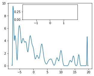
def make_system(a=1, t_1=1.0, t_2=1.0, L=10, r=3):
def circle(pos):
(x, y) = pos
rsq = x**2 + y**2
return rsq < r**2
# return x>=-L//2 and x<<L//2 and y<=L//2 and y>=-L//2
# lat = kwant.lattice.Polyatomic([[3*a/2, np.sqrt(3)*a/2], [3*a/2, -np.sqrt(3)*a/2]], [[0, 0], [a,0]])
R = np.array([[np.sqrt(3) / 2, 1 / 2], [-1 / 2, np.sqrt(3) / 2]])
v_1 = [3 * a / 2, np.sqrt(3) * a / 2]
v_2 = [3 * a / 2, -np.sqrt(3) * a / 2]
r_1 = [0, 0]
r_2 = [a, 0]
lat = kwant.lattice.Polyatomic(
[np.dot(R, v_1), np.dot(R, v_2)], [np.dot(R, r_1), np.dot(R, r_2)], norbs=1
)
lat.a, lat.b = lat.sublattices
syst = kwant.Builder()
onsite = 0
# Onsites
syst[(lat.a(n, m) for n in range(L) for m in range(L))] = onsite
syst[(lat.b(n, m) for n in range(L) for m in range(L))] = onsite
# Hopping
hoppings = (
((0, a), lat.a, lat.b),
((a, 0), lat.a, lat.b),
((-a / 2, -np.sqrt(3) * a / 2), lat.a, lat.b),
((-a / 2, np.sqrt(3) * a / 2), lat.a, lat.b),
)
syst[[kwant.builder.HoppingKind(*hopping) for hopping in hoppings]] = t_1
hoppings2_a = (
((0, a), lat.a, lat.a),
((a, 0), lat.a, lat.a),
((a, -a), lat.a, lat.a),
)
# hoppings2_a = (((a/2, 3*a/2), lat.a, lat.a))
hoppings2_b = (
((0, a), lat.b, lat.b),
((a, 0), lat.b, lat.b),
((a, -a), lat.b, lat.b),
)
syst[[kwant.builder.HoppingKind(*hopping) for hopping in hoppings2_a]] = t_2
syst[[kwant.builder.HoppingKind(*hopping) for hopping in hoppings2_b]] = t_2
LEADS = True
if LEADS:
# Right lead
sym_right_lead = kwant.TranslationalSymmetry(
np.dot(R, [-3 * a / 2, -np.sqrt(3) * a / 2])
)
# sym_right_lead = kwant.TranslationalSymmetry([2*a,0])
right_lead = kwant.Builder(sym_right_lead)
right_lead[(lat.a(n, m) for n in range(L) for m in range(L))] = onsite
right_lead[(lat.b(n, m) for n in range(L) for m in range(L))] = onsite
# Hopping
right_lead[[kwant.builder.HoppingKind(*hopping) for hopping in hoppings]] = t_1
right_lead[
[kwant.builder.HoppingKind(*hopping) for hopping in hoppings2_a]
] = t_2
right_lead[
[kwant.builder.HoppingKind(*hopping) for hopping in hoppings2_b]
] = t_2
syst.attach_lead(right_lead)
right_lead_fin = right_lead.finalized()
syst.attach_lead(right_lead.reversed())
syst_fin = syst.finalized()
if LEADS:
return syst_fin, right_lead_fin
else:
return syst_fin
def plot_bandstructure(flead, momenta, label=None, title=None):
bands = kwant.physics.Bands(flead)
energies = [bands(k) for k in momenta]
plt.figure()
plt.title(title)
plt.plot(momenta, energies, label=label)
plt.xlabel("momentum [(lattice constant)^-1]")
plt.ylabel("energy [t]")
def plot_conductance(syst, energies):
# Compute conductance
data = []
for energy in energies:
smatrix = kwant.smatrix(syst, energy)
data.append(smatrix.transmission(1, 0))
plt.figure()
plt.plot(energies, data)
plt.xlabel("energy [t]")
plt.ylabel("conductance [e^2/h]")
plt.show()
def plot_density(sys, ener, it=-1):
wf = kwant.wave_function(sys, energy=ener)
t = np.shape(wf(0))
nwf = wf(0)[0] * 0
for i in range(t[0] // 2 + 1):
test = wf(0)[i]
nwf += test
psi = abs(nwf) ** 2
if it == -1:
title = "density"
elif it > -1:
title = "density"
title2 = title + ".pdf"
kwant.plotter.map(sys, psi, method="linear", vmin=0)
J_0 = kwant.operator.Current(sys)
c = J_0(nwf)
kwant.plotter.current(sys, c)
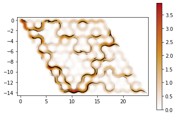
plt.close()Equally easy Kwant enable us to draw full energy spectrum and conductance for sample.
def plot_spectrum(t_1, t_2, c):
    # t_2 = t_2 * np.exp(1j*c)
    sys, right_lead = make_system(t_1=t_1, t_2=t_2 * np.exp(1j * c))
    plot_bandstructure(
        right_lead, np.linspace(-np.pi, np.pi, 100), t_2, title=f"t_1 = 1, t_2 = {t_2}"
    )


# interact(plot_spectrum,t_1=(0.0,5,0.1),t_2=(0.0,5,0.1),c=(-np.pi,np.pi,0.1))
plot_spectrum(1, 0.05, 0)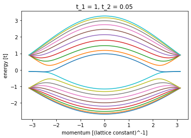
def plot_conductance(t_1, t_2, c):
    sys, right_lead = make_system(t_1=t_1, t_2=t_2 * np.exp(1j * c))
    plot_density(sys, 1)


# interact(plot_conductance,t_1=(0.0,5,0.1),t_2=(0.0,5,0.1),c=(-np.pi,np.pi,0.1))
plot_conductance(1, 0.05, 0)
/usr/local/anaconda3/envs/kwant/lib/python3.6/site-packages/ipykernel_launcher.py:109: RuntimeWarning: The plotted data contains 0.87% of values overflowing upper limit 1.3598 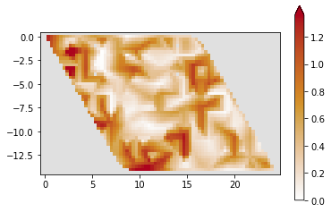
/usr/local/anaconda3/envs/kwant/lib/python3.6/site-packages/ipykernel_launcher.py:114: VisibleDeprecationWarning: Creating an ndarray from ragged nested sequences (which is a list-or-tuple of lists-or-tuples-or ndarrays with different lengths or shapes) is deprecated. If you meant to do this, you must specify 'dtype=object' when creating the ndarraydef plot_probability(ham):
phi_tab = np.linspace(0, 2 * np.pi, 10)
energies = []
for phi in phi_tab:
sys = make_system(t_1=1, t_2=np.exp(1j * phi))
ham = sys.hamiltonian_submatrix(sparse=True)
e_val, e_vec = scipy.sparse.linalg.eigsh(ham, k=197, return_eigenvectors=True)
e_val = np.sort(e_val)
energies.append(e_val)
plt.figure()
plt.plot(phi_tab, energies)
plt.xlabel("t2")
plt.ylabel("energy [t]")
plt.show()
syst = make_system_noleads(a=1, t_1=1, t_2=5 * np.exp(1j * 2), L=5, r=3)
hamiltonian = syst.hamiltonian_submatrix(sparse=False)
plot_probability(hamiltonian)--------------------------------------------------------------------------- AttributeError Traceback (most recent call last) <ipython-input-21-759cfc27acd2> in <module> 17 syst = make_system_noleads(a=1, t_1=1, t_2=5*np.exp(1j*2), L=5, r=3) 18 hamiltonian = syst.hamiltonian_submatrix(sparse=False) ---> 19 plot_probability(hamiltonian) 20 <ipython-input-21-759cfc27acd2> in plot_probability(ham) 4 for phi in phi_tab: 5 sys = make_system(t_1 = 1, t_2 = np.exp(1j*phi)) ----> 6 ham = sys.hamiltonian_submatrix(sparse=True) 7 e_val, e_vec = scipy.sparse.linalg.eigsh(ham, k=197, return_eigenvectors=True) 8 e_val = np.sort(e_val) AttributeError: 'tuple' object has no attribute 'hamiltonian_submatrix'