One Dimensional Scattering – Kwant as a playground for learning quantum transport

In this tutorial, we will explore how to simulate one-dimensional scattering in a lattice. We will walk through the steps to create a lattice system, calculate the transmission probability, and compare the results with analytical solutions. This system can possibly be realized as GaAs nanowire, and this model uses numerical parameters (efective mass and lattice constant), equal to those of GaAs.

import kwant
import matplotlib.pyplot as plt
import numpy as np

First, let’s define useful constants and the function for analytical solutions. It calculates the transmission probability for a given energy \(E\), potential barrier height \(V_0\), and the length of the system \(L\).

JtomeV = 6.242 * 10**21
mevtoJ = JtomeV ** (-1)
hbar = 1.0545718 * 10 ** (-34)  # m^2 kg/s
hbarr = 6.58211 * 10 ** (-13)  # meV s
me = 9.10938356 * 10 ** (-31)  # kg
mc = 1.782 * 10 ** (-36)  ##eV/c^2 = mc kg
c = 3 * 10**8
a = 0.5 * 10 ** (-9)  # m
meff = 0.07  # non dim
t = (hbar) ** 2 / (2 * meff * me * a**2) * JtomeV  # j->mev
l = 5 * 10 ** (-8)
L = int(l / a)
v0 = 20


def an_sol(E, V0=v0, L=0.8 * l):
    E = np.array(E) * mevtoJ
    V0 *= mevtoJ
    m = me * meff
    k2 = np.sqrt(abs(2 * m * (E - V0)) * hbar ** (-2))
    v = []

    for i in range(np.size(E)):
        kd = k2[i]
        e = E[i]
        if E[i] < 0.999999 * V0:
            t = V0**2 * np.sinh(kd * L) ** 2 / (4 * e * (V0 - e))
            v.append(t)
        elif E[i] > 1.0000001 * V0:
            t = V0**2 * np.sin(kd * L) ** 2 / (4 * e * (e - V0))
            v.append(t)
    v = np.array(v)
    return 1 / (1 + v)

Let’s also introduce a piecewise potential function. The potential is zero outside the interval \([p, k]\) and takes the value \(V\) within that interval.

def v(x, p=L / 10.0, k=9 * (L / 10.0), V=v0):
    if x < p:
        return 0
    if x >= p and x <= k:
        return V
    if x > k:
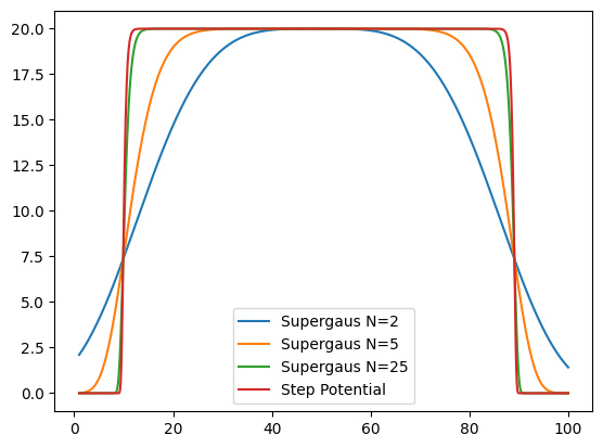
        return 0

We will also make use of the following function that returns a gaussian potential at position \(x\). It has the amplitude \(V\), and width \(w\).

def v_g(x, v=v0, w=2 * L / 5.0, N=50, V=v0):
    return V * np.exp(-(((x - L / 2.0) / w) ** (2*N)))

Here we define the system in a usual way: - we define hoppings and leads - attach leads to the lattice

def make_syst(n):

    syst = kwant.Builder()
    lat = kwant.lattice.chain(a)

    # build
    for i in range(L):
        if n != "inf":
            syst[lat(i)] = 2 * t + v_g(i, N=n)
        else:
            syst[lat(i)] = 2 * t + v(i)

        # hopping
        if i > 0:
            syst[lat(i), lat(i - 1)] = -t

    # left lead
    sym_left_lead = kwant.TranslationalSymmetry([-a])
    left_lead = kwant.Builder(sym_left_lead)
    left_lead[lat(0)] = 2 * t
    left_lead[lat(0), lat(1)] = -t
    syst.attach_lead(left_lead)

    # right lead
    sym_right_lead = kwant.TranslationalSymmetry([a])
    right_lead = kwant.Builder(sym_right_lead)
    right_lead[lat(0)] = 2 * t
    right_lead[lat(0), lat(1)] = -t
    syst.attach_lead(right_lead)
    right_lead = right_lead.finalized()

    # kwant.plot(syst)
    syst = syst.finalized()

    return syst

Now let’s try to calculate the transmission probability (conductance) with respect to energy. We will compare the outputs of Kwant with analytical solutions.

data = []

n = 80
Emax = 3 * v0
energy = np.linspace(0.01, Emax, n)

res = []

# for i in [2,5,20,50]:

for i in [2, 5, "inf"]:
    res_i = []
    syst = make_syst(i)
    for ie in energy:
        smatrix = kwant.smatrix(syst, ie)
        res_i.append(smatrix.transmission(1, 0))

    plt.scatter(energy, res_i, label="KWANT SG n=" + str(i))
    res.append(res_i)


energy = np.linspace(0.001, Emax, 10000)
t = an_sol(energy)
plt.plot(energy, t, label="ANALITICAL")

plt.xlabel("energy [meV]")
plt.ylabel("conductance [e^2/h]")

plt.legend()
plt.show()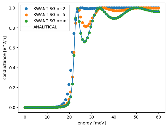

We can see the agreement with theory increses with the Supergausian n parameter. It can be well understood, when comparing diffrent n supergausian potentials with step potential.

i = np.arange(1, 100.1, 0.1)
plt.plot(i, v_g(i, N=2), label="Supergaus N=2")
plt.plot(i, v_g(i, N=5), label="Supergaus N=5")
plt.plot(i, v_g(i, N=25), label="Supergaus N=25")
plt.plot(i, v_g(i), label="Step Potential")

plt.legend()